Build supplement to Part IIOne state, two consequences
One Cut, Two Consequences
From a single free-fermion state, an approximate geometry and a compact, integrated module — both read off the same entanglement, and found to track one another.
The theory and its first toy → Bounded Continuity
r = 0.94. So in this model the same entanglement structure that fixes where things are also tracks which regions read as bounded, integrated subjects. That is the claim, and its limit. This is evidence for the structural plausibility of the Bounded Continuity picture — a careful computational-physics toy — not a proof of it. It recovers an approximate geometry, not emergent spacetime; a compact modular region, not a literal Markov blanket or a felt subject. Seven pass/fail gates are stated; all seven pass. What it does not show — emergent spacetime, dynamics, gravity, cosmology, conditional-independence boundaries, and felt quality — is named as plainly as what it does.
Part I
The state, and why it is finishable
I.1 · The claim to demonstrate
Space and subjects from one factorization
The theory's foundational move is that one factorization, selected for quasiclassicality, produces space, time, and the partition into subjects as a single emergence rather than three. The toy never showed this — it had a subject and an environment but no spatial structure to speak of. The single most valuable thing a follow-on can do is exhibit two of those consequences in one state and show they coincide: recover a geometry from entanglement, and show that a region which makes a good subject — strongly integrated within, controllably bounded across its edge — is also a geometrically localized patch in that same geometry. If both hold in one model, “one cut, two consequences” stops being a slogan and becomes a calculation.
I.2 · Why free-fermion states
The choice that makes it tractable
The decisive practical choice is the class of states. The toy used interacting Heisenberg rings, bound to exact diagonalization and dead near twenty spins — far too small for a geometry to be defined. This model uses free-fermion (Gaussian) ground states of a hopping Hamiltonian H = −t Σ c_i† c_j + m Σ s_i n_i. For any such state every entropy — and so every mutual information — follows from the two-point correlation matrix C_ij = ⟨c_i† c_j⟩ by diagonalizing a submatrix (the Peschel construction): S(A) = −Σ [ν log₂ ν + (1−ν) log₂(1−ν)] over the eigenvalues ν of C restricted to A. This scales to hundreds of sites on a laptop; the largest run here is a 382-site tree, in seconds. That is the step that buys the system sizes a geometry needs to even be definable.
The staggered mass m matters. It opens a spectral gap, so correlations — and the mutual information — decay exponentially with lattice distance. With an exponential decay the distance map d = −log I is linear in lattice distance and the recovered metric is faithful; a gapless state decays polynomially, so −log I ∼ log r and the embedding warps into spuriously high dimension. The gap is what makes “geometry from entanglement” clean, and it is the same reason area-law states and tensor networks carry geometry at all.
I.3 · The ground-truth geometries
A line, a sheet, and a tree
Three lattices serve as known geometries to test recovery against: a line (1D chain; expected dimension ≈ 1, curvature ≈ 0), a grid (2D square lattice; dimension ≈ 2, curvature ≈ 0), and a tree (regular Bethe lattice; negatively curved, no finite dimension). A regular {p,q} Poincaré-disk tiling would be the textbook hyperbolic case; it is not used here, and the reason is worth stating plainly: a naive reflection tiling accumulates floating-point error past the first ring of tiles, and a clean tiling needs exact group arithmetic that is a project in itself. The tree is used instead because it is exact and drift-free, and because it is not a toy substitute — the Bruhat–Tits tree is precisely the bulk geometry of p-adic AdS/CFT, so a regular tree is a legitimate discrete hyperbolic, indeed holographic, space. The claim being tested — recover negative curvature from entanglement and tell it from flat — is served by any genuinely negatively curved graph, and the tree is the cleanest available. Promoting it to a true tiling is the obvious next refinement.
Part II
Recovering the geometry
One caveat before any of the numbers, since it governs how they should be read: the lattice here is local by construction. The model recovers, from mutual information, the geometry it was built on; it does not derive locality, or a quasiclassical factorisation, from a structureless global state — which is the move the full theory would need. That is a real consistency check, not the strong claim, and stating it here (rather than only in Part V) is meant to keep the recovery from being over-read as “spacetime from nothing.”
II.1 · From mutual information to a metric
A graph of mutual information, then geodesics
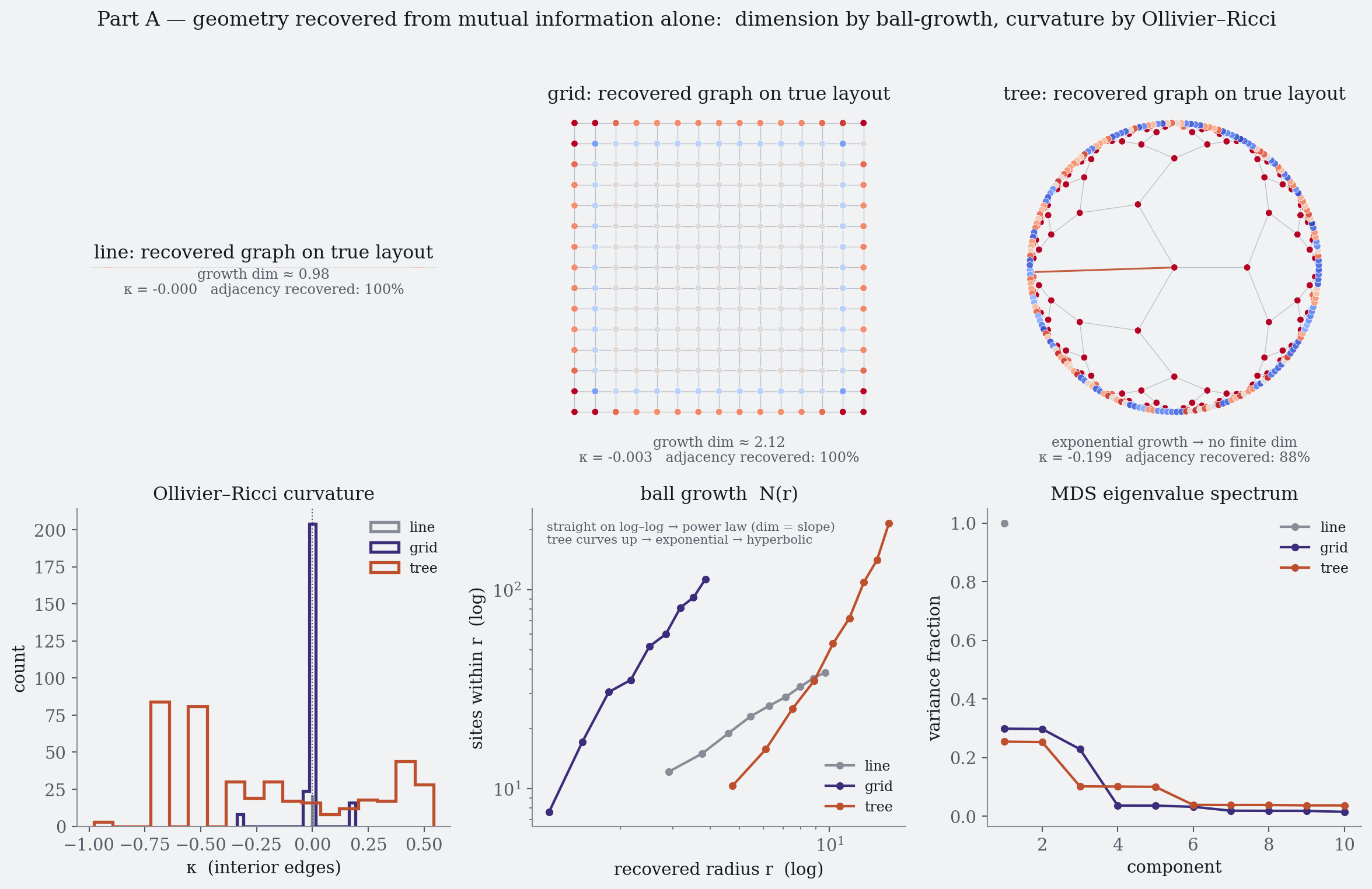
One precision first: the quantity used throughout is the mutual information, which captures total correlations, not entanglement alone. In a pure ground state it is the standard geometric proxy (and the curvature result is cross-checked against a genuine entanglement monotone), so where the prose says “from entanglement” it should be read as “from the mutual-information / correlation structure.” From the correlation matrix, then, the full pairwise single-site mutual information I(i:j) = S_i + S_j − S_ij is computed, and links are kept whose value exceeds a fraction of the global maximum. With a gap the lattice is near-translation-invariant, so the nearest-neighbour shell sits at ≈ max while the next shell collapses far below it; one global threshold therefore recovers the local neighbourhood on any lattice without being told its coordination number. On the line and grid this recovers the adjacency exactly (100%); on the tree, 88%, the residue being links between sibling leaves. Distant pairs get no edge — their separation is recovered as a geodesic on the weighted graph, exactly as Isomap does.
II.2 · Dimension and curvature
Ball-growth and Ollivier–Ricci
Dimension is read by counting how many sites fall within recovered geodesic radius r: for a flat d-dimensional space N(r) ∼ r^d, so d = d log N / d log r — robust to the Manhattan-versus-Euclidean distortion that inflates a naive embedding of a square lattice. For a tree, N(r) grows exponentially, the fitted slope keeps climbing, and no finite dimension exists, which is itself the operational signature of negative curvature. Curvature is read by Ollivier–Ricci on the weighted graph — κ(x,y) = 1 − W₁(m_x,m_y)/d(x,y), with W₁ the optimal-transport distance by linear programming — needing no embedding and cleanly separating flat from negatively curved networks.
Recovered: line 0.98, grid 2.12; the tree's log N(r)-versus-r fit is straight at R² = 0.995 (exponential growth, no finite dimension). Mean interior curvature: line −0.000, grid −0.003, tree −0.199 — flat lattices near zero, the tree decisively negative. Replacing d = −log I with d = √(−log I) leaves the grid dimension near 2 and the tree clearly negative: the geometry is not an artefact of the particular distance map.
Part III
The subject in the same state
III.1 · The boundary and three integration measures
A Markov-blanket-inspired boundary, ported onto the lattice
In the same class of state a contiguous region S is scored with the toy's own measures. The boundary openness O(S) = I(S:E) is the mutual information crossing the cut — the information that leaks between the region and the rest, which rises as the boundary opens. (This is a Markov-blanket-inspired proxy, not a literal Markov blanket: a true blanket is a conditional-independence screening-off, a stronger condition the bare mutual information does not establish — see Part V.) Interior integration Φ(S) is read three ways that should agree: the toy's minimum-information-bipartition proxy; the Fiedler value (algebraic connectivity) of the interior graph, a spectral measure of how hard the interior is to cut; and the fermionic logarithmic negativity, a genuine mixed-state entanglement monotone, computed exactly. A boundary parameter g scales the hopping across ∂S; an interior parameter J_S scales the hopping within.
III.2 · The bending window
Sealed, continuous, recombined
Sweeping g reproduces the toy's three regimes. At g = 0 the subject is sealed: openness O = 0 exactly and Φ is maximal. As g rises the boundary opens (O climbs) while the interior stays integrated; pushed far enough, the boundary bonds dominate, the interior sites pair off with their exterior partners, and Φ erodes — the recombination limit. One honest difference from the toy: here Φ declines smoothly rather than holding a flat plateau, because the free-fermion interior has no rigid closed-shell to protect it. The structure is intact, and all three integration measures track one another — the exact fermionic negativity follows the mutual-information proxy at correlation 0.99, so the trade-off is no artefact of using a correlation measure rather than an entanglement measure.
Varying J_S confirms the one prediction that distinguishes the theory from a simple, one-axis deflationary account: a stronger interior widens the window. The coupling at which Φ falls below threshold moves outward monotonically — g* = 0.55, 1.02, 1.72, 2.42 for J_S = 0.6, 1.0, 1.6, 2.4. A more strongly integrated subject can open its boundary further before it comes apart.
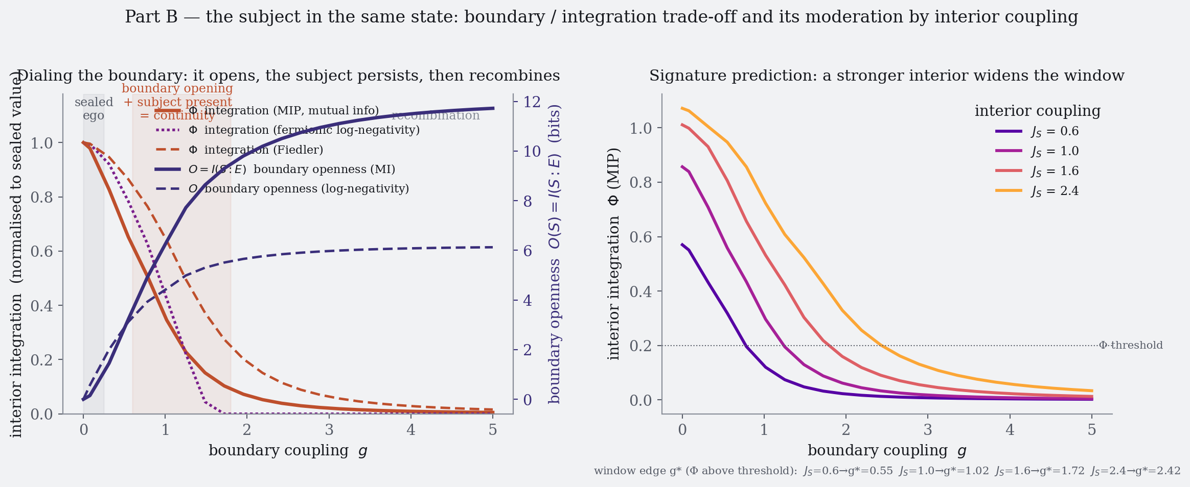
r = 0.99). A stronger interior coupling widens the window — the theory's signature prediction.Part IV
The bridge — the payoff
IV.1 · Subjecthood against compactness
Good subjects are compact patches
Parts II and III are each individually modest. The result that makes the model is the join, computed in the same uniform ground state used to recover the geometry. For many candidate regions of equal size — compact geodesic balls, scattered random sets, and two-blob “split” sets — each is scored on subject-quality Q = internal binding / boundary leakage = (Σ I(i:j) inside) / I(S:E), the Markov-blanket criterion that a good subject talks to itself far more than to the outside; and on geometric compactness K = minus the mean pairwise recovered distance, read purely from Part II's emergent metric.
The two track each other at Pearson r = 0.94. Geodesic balls score high on both (mean Q = 0.45), scattered sets low on both (0.02), two-blob sets in between (0.27). The regions that make good modules are exactly the compact patches of the recovered space. That correlation is the structural claim in one plot: in this model the same entanglement structure that fixes where things are also tracks which regions read as bounded, integrated subjects, and those regions sit at localized places in the space. Two caveats in the spirit of candour. First, Q and K both derive from the one mutual-information structure, so they are not independent variables — but that is the point, not a confound: the claim was never that two separate things happen to correlate, only that a single factorization has these two faces at once. Second, “subject” here is read off low boundary information and high interior integration; calling such a module a subject is the theory's interpretation, not something the calculation establishes.
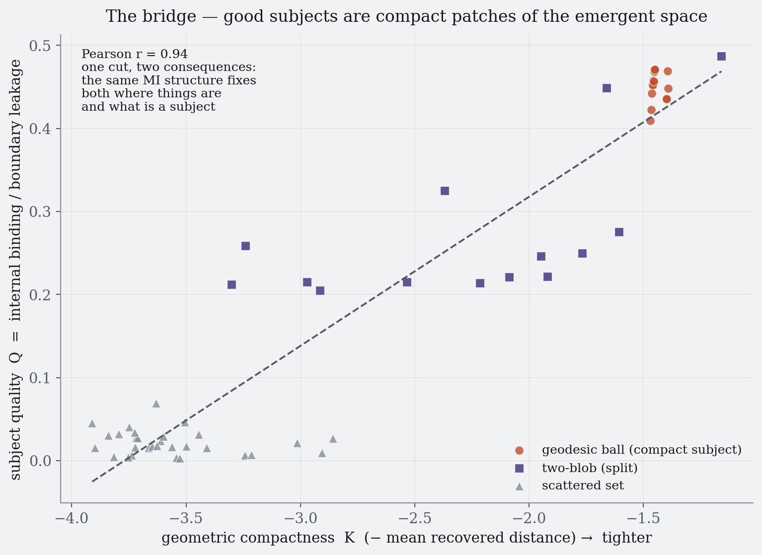
r = 0.94: the regions that make good subjects are the compact geodesic balls of the recovered geometry. One cut, two consequences.Part V
What would sink it, and what it does not show
V.1 · The gates
Seven pass/fail tests, all passed
Built as internal pass/fail gates — sanity and robustness checks for the model, in the series' habit of saying what would sink it. (They validate the toy: they are not an empirical falsification of the theory, which only the brain experiment in Part III could attempt.) The Ollivier–Ricci routine is separately validated against analytic cases (path, cycle, tree, complete graph), and the fermionic-negativity routine against the pure-state Rényi-½ identity and the product-state zero limit, before use.
Dimension separates line (0.98) from grid (2.12). Curvature separates flat (grid −0.003) from hyperbolic (tree −0.199). The tree shows exponential, not power-law, growth (R² = 0.995). The geometry is robust to the distance map. The window widens with interior integration (g*: 0.55 → 2.42). The interior window survives under the exact fermionic log-negativity (correlation with the mutual-information proxy 0.99). And good subjects are geometrically compact (r = 0.94).
recovered dimension or curvature did not converge or flipped under a different distance map; the window vanished or decorrelated across measures; or subject-quality and emergent-spatial compactness had been uncorrelated — a genuine negative result, and worth reporting as one.
V.2 · The limits
What is grounded, and what is not
Stated up front so the model is not over-read.
- Geometry read back from a local Hamiltonian — not locality derived from a structureless Hilbert space. The most important scope limit. The hopping Hamiltonian is local by construction: the lattice is put in by hand, and the model recovers, from mutual information, the geometry it was built on. That is a real consistency check — the metric was not handed to the recovery algorithm — but it is not the theory's own move, which is to have locality and a quasiclassical factorisation selected out of a structureless global state. The model assumes the local structure the full theory would need to derive. So it shows that given locality, entanglement encodes a recoverable geometry; it does not show spacetime emerges from entanglement. The strong claim (à la Ryu–Takayanagi and holographic reconstruction) is separate and far stronger, and the model only gestures at it.
- No dynamics, no gravity. This recovers a static geometry, not one obeying Einstein's equations. The next rung is Jacobson-style emergence — the linearized field equations as an entanglement-equilibrium condition — which needs an entanglement first law the model does not attempt. No cosmology and no de Sitter solution either; that is frontier quantum gravity, independent of any theory of consciousness.
- Boundary openness, not a literal Markov blanket.
O(S) = I(S:E)measures how much information crosses the cut — it rises as the boundary opens, so it is openness/leakage, not a “strength” or closure. And a genuine Markov blanket is more than lowO: it is a conditional-independence structure (interior screened from exterior given the blanket). Establishing that needs additional machinery — a designated blanket layer and a test that interior and exterior are conditionally independent given it — which this model does not implement. “Markov blanket” here is an inspiration for reading off a boundary, not a proven screening-off. - No felt quality. As the toy already conceded, the model tests the structural claims — boundary, integration, localization — and produces no experience. Identifying an integrated, compact module with a subject is the theory's reading; whether such an interior simply is experience is the hard problem, and it sits untouched.
- Honest deviations from the ideal. The hyperbolic case is a regular tree, not a regular
{p,q}tiling. The interiorΦdeclines smoothly rather than holding the toy's plateau. The interior negativity is exact but on a small (seven-site) region, since the exact construction is exponential in region size; a Gaussian closed-form would let it scale. None is a gap in the claim — only places the implementation could be sharpened.
So the honest summary is modest and worth stating in one line: this is a careful computational-physics toy that supports the structural plausibility of the Bounded Continuity picture — mutual information can recover approximate geometry, pick out compact modular regions, and reproduce a boundary/integration trade-off in one state — and it is not a derivation of consciousness, a proof of emergent spacetime, or a literal Markov blanket. It turns one more of the theory's structural claims into a calculation that could have failed, and did not. That is all it does, and it is enough to be interesting.
Elsewhere in the series
Bounded Continuity
The formalism this model extends: a selected factorization, a Markov-blanket boundary, and the original eight-qubit toy whose subject this state finally gives a space to live in.
Part III · The empirical companionThe Window
The single experiment whose result separates this theory from the deflationary account, built on the very interaction this model derives.
Part I · The essayThe Weave and the Window
The plain-language picture: reality as one weave of connection, parsed by a finite point of view.
Appendix · The CorpusData supplement
5,623 near-death testimonies scored item-by-item against the wager — the empirical ledger behind the series.